An overview of LBNL Radiance for annual daylight analysis
A brief overview of LBNL Radiance
The following is an adaptation in article form (and translation from Italian to English), of a literature review I had lying on my hard drive. Since there it has no use, I decided to publish it here.
I hope it can serve as a general overview of the Radiance software suite, targeted to numerical annual daylight analysis, for those who are starting out, before diving into the technical details, well explained in the documentation available online (a selection of which is written at the end of the article and referenced throughout).
Introduction
The problem
Today the construction sector pays a lot of attention to energy efficiency in buildings. In this scenario, quantifying daylight becomes particularly relevant.
The output of interest is not an image, even if it’s possible to create them, but illuminance values computed for a typical year in the hours of occupancy of the rooms, in “sensor points” placed on the horizontal work plane.
Why Radiance
Radiance is a suite of open-source software maintained by the LBNL (Lawrence Berkeley National Laboratory, University of California) since the nineties.
Thanks to the capability to specify virtually any mesh and material, to the numerous validations (both comparing Radiance with other software and with real-world and to scale measurements), to the possibility to perform point in time and annual simulations, to evaluate illuminance, daylight factor, glare, etc. Radiance is to this day the standard adopted by the construction industry.
Operative System
Premise (choice of the operative system)
“native” software is written in a programming language (C for example) so that the developer can instruct the computer on the logic to be executed in a human-readable syntax. The processor though doesn’t understand what the developer writes, it only understands machine code (sequences of binary). So a specific software is necessary to translate from one language to the other, called a compiler.
The C language is the same for everyone, but the machine code is processor-specific.
Radiance is originally written and compiled for UNIX-type operative systems (Linux and macOS). Being open-source is possible to browse and download C code and compile it personally. If you don’t care about it, NREL provides precompiled versions for Linux, macOS, and Windows (5.3 is available at the time of writing).
The Windows version has limited capabilities, both in the availability of certain executables and in the exploitation of modern processors’ multi-core performance, but it’s nice to be integrated into commercial engineering software, that usually runs on Windows.
You can use the Linux version on Windows 10 using WSL, here is the link to an article about how to do that I previously wrote: Linux Radiance on Windows with WSL and X11.
There’s also an interesting MIT project named Accelerad, which has adapted the Radiance raytracing engines (rtrace, rpict, rfluxmtx, etc.) to run on modern Nvidia graphics cards that support OptiX and CUDA. The advantage of using a GPU over a CPU for raytracing calculation is that GPUs are optimized to make a lot of operations in parallel, matrix multiplication in particular.
The following is a table that compares the OSs:
| Windows | macOS | Linux | |
| System preinstalled on a computer | X | X (on iMac and MacBook) | |
| Based on UNIX | X | X | |
| Multicore operations | X | X | |
| Widespread CAD software to export geometry | X | X (limited) | X (very limited) |
| Cloud computation | X |
I would say that for a single user for which daylight analysis is an important activity, macOS is the easiest solution.
Windows (especially in conjunction with WSL or Accelerad) is the best alternative for the user that doesn’t only do daylight, and fancies using commercial CAD software.
The advanced user which is building (or renting in the cloud) a machine to specifically run Radiance, and has other machines to run other software, should definitely use Linux.
The terminal
Reference [1] UNIX for Radiance – Axel Jacobs – 2010
When you’ve chosen the OS and installed the relevant Radiance version, the interface with the software is the command line (aka the terminal, aka the system console).
What follows in the article, if not differently specified, uses UNIX syntax (the one used in most of the documentation).
The terminal is a text interface that allows us to interpret and execute bash commands or shell scripts.
Useful general commands include:
pwd [print working directory]: prints the current directory;cd [change directory]: followed by a directory path, brings to it;ls [list]: prints a list of the sub-directories (subfolders or files) of the current directory;cat [concatenate]: prints the result of the operation that follows it (the content of a file, results of algebraic expressions, or output of other commands).
Useful key combinations include:
Enter: executes operations written in the command line;Ctrl [Cmd] + C: aborts the operation in execution;Tab: auto-complete;Top/Down Arrow: loops through recently used commands in order of execution;Mouse Right Click: Paste.
The general syntax for a command is:
std_input < program_1 -flag1 -flag2 -flagN | program_2 -flag1 -flag2 -flagN > std_output
With an analogy with math, a program is like a function, and flags are like the function’s parameters (constant or variable).
Input (scene description)
All the files with which Radiance interacts are simple text files (.txt). For user comfort, it’s usual to substitute the .txt extension with .rad, .mat, .rif, .vf, .sky, etc. to better understand the content without opening the file. At their roots, they’re still text files.
Geometry
Reference [2] Radiance Primer – Giulio Antonutto and Andrew McNeil
Radiance uses a right-handed cartesian 3d space, where the XY plane represents the horizontal plane at altitude zero, the positive Z-axis indicates increasing altitude. The positive X-axis coincides with the east direction, the Y-axis with the north, and so on.
Lengths can be expressed in any unit, as long as it is consistent across all files of a given project. For buildings, it’s advised to express everything in meters.
Geometry is specified with the format:
modifier type name
ns s1 s2 sN
ni i1 i2 iN
nf f1 f2 fN
where:
modifier: is the material assigned to a surface
type: is the primitive type
name: is an alphanumeric string without spaces that uniquely identifies the surface (ex. sup123). It can be a random number, the typical situation when the surface is automatically generated by a CAD application
ns: number of string parameters (an ex. of a string is “hello_world”)
s1 s2 sN: the string parameters
ni: number of integer parameters (an ex. of an integer is 123)
i1 i2 iN: the integer parameters
nf: number of float parameters (an ex. of a float is 123.45)
f1 f2 fN: the float parameters
For example, a triangle with a material named matte_red would be:
matte_red polygon triangle1
0
0
9 0 0 0
10.5 0 0
10 10.3 0
Float type parameters can contain integers. Every line represents the coordinates X Y Z of the point of the polygon.
The most used primitives are:
polygon: a polygon is described by a list of coplanar vertices in 3d space, in counterclockwise order if seen from the front of the face (where the normal points). The last vertex is automatically connected to the first one. Holes are represented by internal vertices, connected to the perimeter with coincident edges (“seams”);source: a source is described by a solid angle. It’s used to define light sources infinitely far away. It’s defined by the distance between the global origin and its center, and by the number of degrees underlying its disc.
The other primitives (less relevant in everyday use) are:
sphere,cone,cup,cylinder,tube,ring
Light and photometric quantities for Radiance
Reference [3] Behavior of Materials in Radiance – Greg Ward – 2004
Reference [4] Radiance Tutorial – Axel Jacobs – 2012
Reference [5] Radiance Cookbook – Axel Jacobs – 2014
Radiance exploits the principles of geometric optics, which models the oscillating nature of light with straight rays.

Light spectrum (by Philip Ronan, Gringer, CC BY-SA 3.0, via Wikimedia Commons)
From the visible radiation spectrum, only three wavelengths are considered, those corresponding to red (670 nm), green (520nm), and blue (460nm).
Radiance
Radiance (the quantity, not the software) or radiation intensity \(R\), is the base radiative quantity, defined as:
$$R = {d^2\phi\over d\Omega dA \cos{\theta}} \quad \left[{W \over {m^2 sr}}\right]$$
where \(\phi\) is the radiative flux that crosses a given surface, \(A\) is the surface, \(\Omega\) is the solid angle between the surface and a hemisphere built around the surface in the direction of the normal, \(\theta\) is the angle between the direction of the radiation and the axis which goes through the Zenit.
Irradiance
Irradiance \(G\) is the incident radiance; it equals:
$$G = \sum_\lambda G_\lambda \quad with \lambda = r: 670nm, g: 520 nm, b: 460 nm \quad \left[{W \over m^2}\right]$$
where \(G_\lambda\) is the monochromatic irradiance defined as:
$$G_\lambda = \alpha_\lambda G_\lambda \cdot \rho_\lambda G_\lambda \cdot \tau_\lambda G_\lambda \quad \left[{W \over {nm m^2}}\right]$$
where \(\alpha_\lambda\), \(\rho_\lambda\) and \(\tau_\lambda\) are respectively the coefficients of absorption, reflection and transmission of the material.
Illuminance
Irradiance in the visible spectrum is called illuminance.
The conversion between irradiance and illuminance is done through the equation:
$$E = K (G_r V_r + G_g V_g + G_b V_b) \quad \left[lux = {lm \over m^2}\right]$$
where \(V_\lambda\) are the coefficients of luminous monochromatic efficiency (\(V_r = 0.265; V_g = 0.670; V_b = 0.065\)) and \(K\) is the luminous efficacy (defined as the ratio between luminous flux and radiative flux), which depends on the source type. Radiance uses \(K = 197 lm/W\).
Radiosity
Radiosity \(J\) is the radiance that leaves a surface; it equals:
$$J = J_{em} + J_r + J_{tr} \quad \left[{W \over m^2}\right]$$
where \(J_{em}\) is the emitted component, \(J_r\) is the reflected component, \(J_{tr}\) is the transmitted component.
Luminance
Radiosity in the visible spectrum is called luminance.
The conversion between radiosity and luminance is done trough the equation:
$$L = K (R_r V_r + R_g V_g + R_b V_b) \quad \left[{cd \over m^2}\right]$$
where \(V_\lambda\) are the coefficients of luminous monochromatic efficiency (\(V_r = 0.265; V_g = 0.670; V_b = 0.065\)) and \(K\) is the luminous efficacy (defined as the ratio between luminous flux and radiative flux), which depends on the source type. Radiance uses \(K = 197 {lm \over W}\).
Materials
Reference [2] Radiance Primer – Giulio Antonutto e Andrew McNeil
Reference [3] Behavior of Materials in Radiance – Greg Ward – 2004
Reference [6] The Radiance 5.1 Synthetic Imaging System – LBNL – 2017
In this paragraph, materials that define luminous sources (for daylight the sun, and the sky) are deliberately omitted, because they’re treated in a following paragraph.
With “material” we mean a function that returns the reflective component of a light ray (represented as a vector coming from a light source). For transparent materials also the transmitted component is returned. It’s a combination of color and reflection (and/or transmission) type.
Since Radiance only samples three wavelengths, materials contain three coefficients of reflection (and transmission if necessary). It is possible to model grey bodies, setting equal values for the coefficients (with this hypothesis if we generated an image, we would see a grayscale picture, hence the name “grey bodies”).
A material is specified with the same format as geometries:
modifier type name
ns s1 s2 sN
ni i1 i2 iN
nf f1 f2 fN
where:
modifier: is the texture (or pattern) assigned to the material. Often this is of no interest, so void is used
type: the material type, which defines the reflection (and/or transmission) type
The main types are:
plastic: is the most common material. These reflections aren’t related to the color, so if a plastic sphere is subject to green light, it will have a green reflection, regardless of the sphere color. It’s specified as:
void plastic name
0
0
5 R G B specularity roughness
R G B parameters are the coefficients of reflection, from 0 (full absorption or black) to 1 (full reflection or white) in the three wavelengths Red, Green, and Blue. They define the color.
specularity
roughness
metal: it’s like plastic, but reflections are related to the color
specularity varies between 0.5 (dirty) and 1 (clean)
roughness varies between 0 (polished) and 0.5 (roughened)
trans: it’s a translucid material. Transmitted and reflected light it’s specified as:
void trans name
0
0
7 R G B specularity roughness transmissivity specular_transmitted_component
specularity varies between 0 (matte) and 0.7 (satin)
roughenss
transmissivity
Transmissivity is defined as:
$$t_n = {\sqrt{0.8402528435 + 0.0072522239 TN^2} – 0.9166530661 \over 0.0036261119 TN}$$
where:
\(t_n\): transmissivity, Radiance parameter
\(TN\): coefficient of visible transmission given by the glass producer (usually called “tau vis”)
specular_transmitted_component is the ratio of transmitted light that isn’t diffused, it varies between 0 (diffuse) and 1 (clear)
dielectric: it’s a transparent material, that refracts light besides reflecting and transmitting it. It’s specified as:
void dielectric name
0
0
5 Rtn Gtn Btn ior hc
Rtn, Gtn, and Btn are the transmissivities for each wavelength
ior is the index of refraction
hc is the Hartmann constant, that modifies the index of refraction depending on the wavelength
glass: it’s a version of dielectric optimized for infinitely thin surfaces (as windows glasses are usually modeled in buildings), with a predefined index of refraction set to 1.52. It’s specified as:
void glass name
0
0
3|4 Rtn Gtn Btn [ior]
BSDF (it deserved its own paragraph so check the next section)
Other types that are less used:
prism, ashik, interface, mirror, mist, antimatter
BSDF
Reference [7] genBSDF Tutorial – Andrew McNeil, LBNL – 2015
Reference [8] BSDF definition – LBNL Window technical documentation chapter 15
BSDF (Bidirectional Scattering Distribution Function) is a material described by a matrix, saved in a .xml file, that is the sum of two matrices:
$$BRDF (Bidirectional Reflectance Distribution Function) + BTDF (Bidirectional Transmittance Distribution Function)$$
The matrix contains coefficients that indicate the direction for reflected rays (BRDF) and transmitted rays (BTDF) for each incident ray direction.
NOTE: The file contains eight separate matrices, four for the visible spectrum, four for the solar spectrum. Of the four matrices, two are for transmission (one from front to back called “transmission front, one from back to front called “transmission back”) and two are for reflection (one from front to front called reflection “front”, one from back to back called “reflection back”).
In particular, the full basis matrix (aka Klems’ basis) is 145 x 145.

BSDF hemispheres (from LBNL Window technical documentation, section 15-2)
The matrix of reflection contains 145 columns, one for each incident ray direction, with 145 elements per column, one for each direction in which a ray can be reflected. A perfectly specular material generates a reflected ray only in one direction; a diffuse one generates many in several directions, here comes the usefulness of BRDF.
Similarly, the transmission matrix contains 145 columns, one for each incident ray direction, with 145 elements per column, one for each direction in which a ray can be transmitted. A perfectly transparent material generates a single transmission ray (this is what happens if you use type glass). So for windows, BTDF is useful when there are elements of obstruction to light penetration, like sunshades, films, or surface treatments that influence light transmission and reflection differently in different directions.

BSDF matrix layout (from LBNL Window technical documentation, section 15-3)
NOTE: more detailed BSDFs can be generated by dividing each patch in half in both directions n-times. There are also dynamic resolution BSDFs, which change the dimension of the patches, putting more detail where there is more variation in data.
More will be said about BSDFs further down the article, as they form the basis for the Matrix simulation methods used in annual daylight simulations.
The sky and the sun
Reference [9] EnergyPlus Version 9.1.0 Documentation Auxiliary Programs – U.S. Department of Energy – 2019
Reference [10] CIE general sky standard defining luminance distribution – Stanislav Darula e Richard Kittler – 2002
In daylight analysis, the only two light sources are the sky and the sun.
Radiance uses two alternative models to define the sky, depending on the simulation you want to perform. For a point in time calculation, the rtrace executable uses the CIE 1994 (produced by gensky), for annual calculation with the multi-phase method rfluxmtx uses Perez’s model (produced by gendaylit).
Sky models output a luminance value for the different points of the sky hemisphere, relative to the Zenit luminance, given latitude, longitude, and hour of the day.
The Zenit value can be retrieved from a .epw (Energy Plus Weather, essentially a .csv) file.
Using .epw files, which are obtained by statistical interpretation of historic weather series, gives a good idea of the annual behavior. If instead, you need to compare your simulation with a real-world measurement taken in a specific setting, you’ll need to know the real weather conditions during the measurements, as statistical data won’t match them.
The continuous sky description gets discretized for annual simulations using the Reinhart model.

Tregenza sky discretization model (on the left) and Reinhart sky discretization model (on the right)
The sun is represented by three or four patches of the discretized hemisphere, or by a geometry of type source and material fo type light, specified as follows:
void light sun
0
0
3 R G B
The sensor plane
A sensor plane is a grid f points in which we want to compute a daylight quantity, usually illuminance. It’s defined in a .pts (points) file.

The sensor plane
The schema of the file is the following row, repeated as many times as there are points:
px py pz nx ny nz
where:
px is the global x coordinate of the point
py is the global y coordinate of the point
pz is the global z coordinate of the point
nx is the component along x of the normal to the plane of the sensor
ny is the component along y of the normal to the plane of the sensor
nz is the component along z of the normal to the plane of the sensor
NOTE: points don’t need to be on a flat plane, they can be in any position pointing in any direction.
For example, a sensor positioned at 76cm from the ground plane, in a 2 x 3 m room, with a 50cm spacing would be:
0.25 2.75 0.76 0.0 0.0 1.0
0.25 0.25 0.76 0.0 0.0 1.0
0.25 1.25 0.76 0.0 0.0 1.0
0.25 0.75 0.76 0.0 0.0 1.0
0.25 1.75 0.76 0.0 0.0 1.0
0.25 2.25 0.76 0.0 0.0 1.0
1.25 1.75 0.76 0.0 0.0 1.0
0.75 0.25 0.76 0.0 0.0 1.0
1.25 2.75 0.76 0.0 0.0 1.0
0.75 1.75 0.76 0.0 0.0 1.0
1.25 0.75 0.76 0.0 0.0 1.0
1.25 0.25 0.76 0.0 0.0 1.0
0.75 2.75 0.76 0.0 0.0 1.0
0.75 2.25 0.76 0.0 0.0 1.0
0.75 0.75 0.76 0.0 0.0 1.0
0.75 1.25 0.76 0.0 0.0 1.0
1.25 1.25 0.76 0.0 0.0 1.0
1.25 2.25 0.76 0.0 0.0 1.0
1.75 1.25 0.76 0.0 0.0 1.0
1.75 0.75 0.76 0.0 0.0 1.0
1.75 2.25 0.76 0.0 0.0 1.0
1.75 0.25 0.76 0.0 0.0 1.0
1.75 1.75 0.76 0.0 0.0 1.0
1.75 2.75 0.76 0.0 0.0 1.0
Computation
Having completed the inputs’ description, there are two types of analysis we can obtain from Radiance computational engines.
Before describing the algorithms and the methods employed, it’s useful to visualize the architecture of the software:

Radiance pipeline
Generator: CAD software from which to export geometry, materials, and light sources.
xform: an executable that modifies geometry files with elementary transformations (translation, rotation, scaling); these operations can be done directly in the CAD application, but they can be useful to merge files exported from different applications (which maybe had a different reference system) or to compose them in arrays.
Scene description: geometry, materials, lights, sensors as described before.
oconv and Octree: oconv is the executable that translates the scene description, in a data structure called Octree, which is a tree diagram where each node has eight branches.
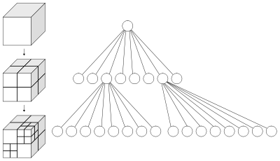
Octree diagram
This structure allows dividing space into octants (one-eighth of the parent space), improving the performance of the computation of intersections between light rays and surfaces, a key step for raytracing.
In short words, the algorithm tests the intersection of the rays with the octants, before testing it with the single polygons. The logic is that if a ray doesn’t intersect with an octant, it will certainly not intersect the polygons that the octant contains, allowing the simulation to skip useless steps.
An octree is a space subdivision system. There are also hierarchical subdivision schemas called Boundary Volume Hierarchy (BVH). These systems generate branches of the tree based on the structure of the polygons. For example, if we wanted to render a bottle, a BVH system would subdivide it into two branches, one for the body, one for the stopper. This allows subdividing the space in a way that’s more adherent to the scene, which can be useful if the density of the objects varies greatly throughout it, but requires the input files to have a hierarchical structure, which requires more setup.
As said, Radiance uses the first system.
Raytracing
Reference [11] The Radiance Photon Map Extension – Roland Schregle – 2019
Reference [12] The Radiance Lighting Simulation and Rendering System
Reference [13] RADIANCE: a simulation tool for daylighting systems – R. Compagnon – 1997
Raytracing is an algorithm that models the real behavior of light, emitting luminous rays from sources and verifying the intersection with the scene’s surfaces, that modify the direction and the intensity of light based on their material.
The reading of the results in the sensor points, or in the pixels of an image, happens when one of these rays passes through them.
It’s immediately clear that this kind of computation would require a huge amount of rays because the probability of one of the rays hitting the sensor points (or the individual pixels) would be pretty low.
This kind of algorithm is known as “forward raytracing” (from source to target).
To reduce the computational effort of such an algorithm we emit rays from the sensor points and trace them back to the light source. If the ray doesn’t find obstructions it means it’s directly lit, otherwise it’s only indirectly lit, so we’ll need to bounce off other surfaces before we get to the light source. This technique makes sure that the sensor will get hit (since it’s the source), so we will get a value no matter what (of course it can be 0 if no light source it’s reached).
This kind of algorithm is known as “backward raytracing” (from target to source).
Radiance (along with most applications of raytracing) makes use of the latter method, although there is an extension called “photon map” that adds the capability to use the former, useful for simulating particularly complex reflections and caustics.
The computation of direct radiation it’s immediate and quick, the indirect one it’s more complex and requires the definition of more parameters to control the simulation.
Let’s quickly go through these parameters and explain what they mean.
NOTE: in the following list, the Radiance flag to define the parameter it’s indicated in square brackets.
- ambient bounces [
-ab]: this is the maximum number of bounces that the raytracer will do to compute indirect illumination; - ambient divisions [
-ad]: this is the number of rays that the main ray will be divided into for each bounce; - ambient value [
-av]: this is a value of radiance that lights up every part of the scene no matter what. It’s like a global light that comes from nowhere but is everywhere. It’s a base indirect illumination value averaged with the indirect calculation. This is compensation for the energy that the raytracer is losing due to its discrete nature. The more rays you compute, the less this is necessary; - ambient weight [-aw]: referring to ambient values, we said it’s an average. Well, this is the weight used for the average between the ambient value and the indirect bounce; 0 means no ambient value;
- ambient accuracy [
-aa]: this indicates how much interpolation happens between computed ambient values. To see this clearly, try to set it to 0 (no interpolation). You’ll see that most of the scene is pitch black (or equal to-avif it’s not set to 0), and some small dots are representing the ambient values. Increasing, even slightly, the accuracy interpolation (for example setting-aa0.1), will cause a circle of light to appear around every ambient value; - ambient resolution [
-ar]: this determines the maximum density of ambient values used in interpolation. The maximum ambient value density is the scene size times the ambient accuracy (see the−aaoption above) divided by the ambient resolution; - ambient sampling [
-as]: this is the number of super samples applied to ray divisions that show a significant change in value. A super sample is an additional subdivision for indirect rays, only in a very small solid angle around it; - limit weight [-lw]: this limits the weight of each ray to a minimum decimal value. If the contribution of a ray to an ambient value is very low, there is no reason to bounce it further;
- limit reflection [-lr]: this limits reflections to a maximum integer number.
Every time a ray hits a surface it has to evaluate the direction of reflection (and transmission if the surface it’s translucent) and the intensity of light ray. It does this by plugging the surface normal (defined by angles) and the material properties in the rendering equation:
$$L_r(\theta_r, \phi_r) = L_e(\theta_r, \phi_r) + \int_{0}^{2\pi} \int_{0}^{\pi} L_i(\theta_i, \phi_i) \rho_{bd}(\theta_i, \phi_i; \theta_r, \phi_r) |cos(\theta_i)| sin(\theta_i) \,d\theta_i \,d\phi_i$$
where:
\(\theta\) is the polar angle (zenithal) measured from the normal of the surface
\(\phi\) is the azimuthal angle measured around the normal of the surface
\(L_e(\theta_r, \phi_r)\) is the emitted radiation in \([{W \over {m^2 sr}}]\)
\(L_r(\theta_r, \phi_r)\) is the reflected radiation
\(L_i(\theta_i, \phi_i)\) is the incident radiation
\(\rho_{bd}(\theta_i, \phi_i; \theta_r, \phi_r)\) is the BRDF (Bidirectional Scattering Distribution Function) in \(sr^{-1}\)
Single-phase method (for point in time analysis): rtrace
The single-phase method solves the problem of computing illuminance on the horizontal plane (previously defined as sensor) using backward raytracing as described in the general case, applied on the whole scene in a single step (hence single phase).
The computation engine is called rtrace.
This approach allows for accurate numerical (often illuminance on a plane) or visual results (to evaluate glare for instance) but requires an entirely new calculation even if few details of the scene change between one simulation and another. A typical case of a minor change in the scene in annual daylight analysis is the variation of the sky luminance distribution.
Matrix-based method (for annual analysis): rfluxmtx
Reference [14] Daylighting Simulations with Radiance using Matrix-based Methods – Sarith Subramaniam – 2017
To account for the problem described at the end of the previous paragraph we introduce the multiphase methods (also called matrix-based methods, for reasons that will be later clear).
Matrix methods compute the illuminance on the horizontal plane using matrices that represent the geometry and materials of the scene, the sky, and the window surfaces. There are six matrix-based methods, that add complexity progressively.
The advantage of this approach is that if only one of the components at play changes, like the sky, we can recompute only the matrix relative to it. The final output in fact isn’t the result of pure raytracing anymore, but of matrices multiplication. If one of them changes, we only need to redo the multiplication, which makes the methods orders of magnitudes faster than using raytracing each time.
This allows us to make annual simulations with multiple configurations.
Two-phases method (or daylight coefficient method) \(\bf E = C_{dc}S\)
Reference [15] Daylight coefficients – Peter Roy Tregenza e I. M. Waters – 1983
The principle is that daylight in a space can be computed considering two independent factors: the luminance of the sky and the optical properties of the scene’s surfaces.
The reference equation is:
$$E = C_{dc} S$$
$$
\begin{bmatrix}
E_1 \\
E_2 \\
\vdots \\
E_n
\end{bmatrix}
=
\begin{bmatrix}
D_{1 1} & D_{1 2} & \cdots & D_{1 m} \\
D_{2 1} & D_{2 2} & \cdots & D_{2 m} \\
\vdots & \vdots & \ddots & \vdots \\
D_{n 1} & D_{n 2} & \cdots & D_{n m}
\end{bmatrix}
\begin{bmatrix}
S_1 \\
S_2 \\
\vdots \\
S_m
\end{bmatrix}
$$
where \(n\) is the number of sensor points (100 for example) and \(m\) is the number of patches of the sky (145 for example).
\(E\) is the illuminance vector (n x 1) where each element is the illuminance computed for each ordered grid point;
\(C_{dc}\) is the matrix of daylight coefficients (n x m) where each element is the coefficient \(D\) of the i-th grid point generated from the j-th sky patch.
The \(D\) coefficient represents:
$$D = R_1 R_2 R_3$$
where:
\(R_1\) is the matrix that defines external obstruction;
\(R_2\) is the matrix that defines direct components;
\(R_3\) is the matrix that defines internal reflections;
Radiance computes \(D\) with raytracing using rfluxmtx.
\(S\) is the sky vector (m x 1) where each element is the luminance of a sky patch.

The sky vector S visualized [1. Continuous distribution (m = \(\infty\)), 2. Reinhart subdivision 1 time (m = 145), 3. Reinhart subdivision 2 times (m = 577), 4. Reinhart subdivision 4 times (m = 2305)]
Three-phases method \(\bf E = V T D S\)
The three-phases method allows specifying complex fenestration systems by adding a transmission matrix \(T\), and separating the luminous flux from the source to the sensor in two fluxes; from the source to the window and from the window to the sensor.
The reference equation is:
$$E = V T D S$$
The \(T\) matrix is simply the BSDF that we already discussed above.
The \(V\) matrix is generated by placing a Klems hemisphere (the hemisphere discretized according to the Reinhart model) on the window facing inwards and generating rays for each patch direction towards the room.

Graphical representation of the view matrix V
Similarly, the matrix \(D\) is generated by placing e Klems hemisphere on the window facing outwards.

Visualization of the daylight matrix D
Four-phases method (with \(\bf F\) matrix) \(\bf E = V T F D S\)
The limitation of the three-phase method is that the transmission method \(T\) only supports pseudo-planar fenestration systems.
The four-phase method introduces further matrices (\(F\), \(FH\), \(FN\) see image below) that allow specifying spatial fenestration systems.
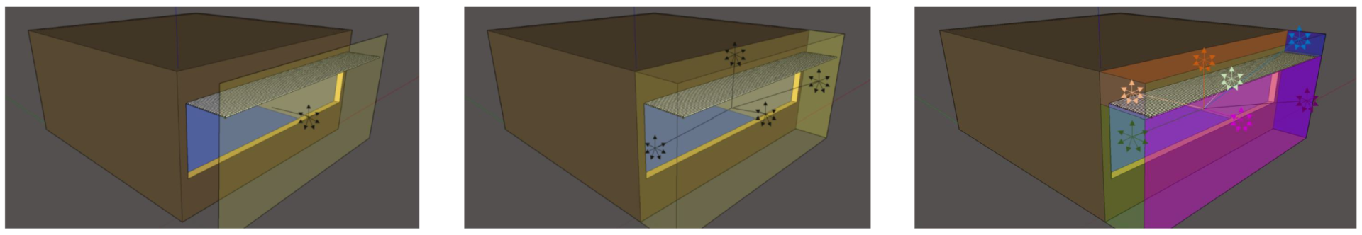
From left to right, the surfaces on which the \(F\), \(FH\) and \(FN\) matrices are assigned to
\(F\) matrices are of BSDF type too.
Two-phases DDS, five and six-phases methods
The two, three, and four-phases methods approximate the Sun to four sky patches. This approximation can be a bit rough. For a more precise computation, the Sun can be modeled separately. This is the goal of the five and six-phases methods, which include the correction of the Sun to the three and four-methods respectively.
The reference equations are respectively:
$$E_{5 phases} = V T D S – V_d T D_d S_d + C_{ds} S_{sun}$$
$$E_{6 phases} = V T F D S – V_d T F_d D_d S_d + C_{ds} S_{sun}$$
The two-phases DDS method (DDS stands for Direct DaySim), introduces the same correction to the two-phase method (the one with daylight coefficients only).
$$E_{DDS} = C_{dc} S – C_{dc d} S_d + C_{sun} S_{sun}$$
NOTE: the \(d\) in the above equations stands for “direct”.
Output
Illuminance file: the time factor (.ill)
The illuminance file in .ill format (that is still a .txt renamed .ill for convenience) is the container of irradiance results (easily convertible in illuminance as seen in an above paragraph).
With this data structure, the time factor is introduced in the simulation. In fact, as said, the matrix methods output a vector \(E\) for each instant of time \(t\) in which the simulation is set to run. It’s sufficient to run the computation varying sky conditions (and the position of the Sun) to have vectors \(E(t)\). By composing the \(E\) vectors in a matrix it’s possible to memorize in a compact and analyzable data structure the input sensors’ annual illuminance profile.
Specifically, the format is:
month day hour row_vector_E
1 1 1.000 0 0 0 0 0 0
1 1 2.000 0 0 0 0 0 0
1 1 3.000 0 0 0 0 0 0
1 1 4.000 0 0 0 0 0 0
1 1 5.000 0 0 0 0 0 0
1 1 6.000 0 0 0 0 0 0
1 1 7.000 0 0 0 0 0 0
1 1 8.000 55 81 92 94
1 1 9.000 813 1777 2368 2592
1 1 10.000 2043 3064 10990 11890
Analysis parameters
Reference [16] Ten key daylight & electric light metrics – Liam Buckley www.iesve.com – 2019
The annual illuminance profile is rich in useful information but, as it stands, is hard to read; so it’s necessary to define parameters to understand it.
Standard Daylight Autonomy e Annual Sunlight Exposure (LEED)
The LEED certification system proposes two parameters:
sDA300lux/50% (standard Daylight Autonomy) is the sufficiency of daylight in a space. It’s defined as the percentage of the analysis area (e.g. the sensor on the horizontal work plane) that reaches a minimum illuminance value (e.g. 300 lux) for a specified fraction of the operative hours of the year (e.g. 50% of the operative hours).
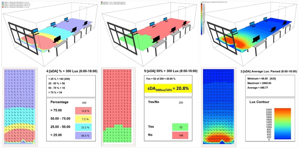
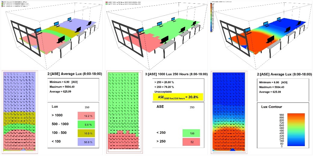
ASE1000lux/250h (Annual Sunlight Exposure) describes the visible potential discomfort in a space. It’s the percentage of the analysis area that exceeds a specified illuminance level (e.g 1000 lux) for a specified number of operative hours of the year (e.g. 250 hours).
Useful Daylight Illuminance
The UDI (Useful Daylight Illuminance) is the percentage of illuminance points (on the sensor plane) that falls in the “usable” range. Values are computed in a predefined range of hours.

The defined ranges for illuminance are:
- Insufficient (below 100 lux): it always requires artificial light;
- Supplementary (between 100 and 500 lux): sometimes it requires artificial light;
- Autonomous (between 500 and 2500 lux): it never requires artificial light;
- Exceedance (above 2500 lux): requires daylight shading systems.
Useful references
- UNIX for Radiance – Axel Jacobs – 2010 | http://www.jaloxa.eu/resources/radiance/documentation/docs/unix4radiance.pdf
- Radiance Primer – Giulio Antonutto e Andrew McNeil | https://radiance-online.org/learning/tutorials/radiance-primer.pdf
- Behavior of Materials in Radiance – Greg Ward – 2004 | https://floyd.lbl.gov/radiance/refer/materials.pdf
- Radiance Tutorial – Axel Jacobs – 2012 | http://www.jaloxa.eu/resources/radiance/documentation/docs/radiance_tutorial.pdf
- Radiance Cookbook – Axel Jacobs – 2014 | http://www.jaloxa.eu/resources/radiance/documentation/docs/radiance_cookbook.pdf
- The Radiance 5.1 Synthetic Imaging System – LBNL – 2017 | https://floyd.lbl.gov/radiance/refer/ray.html
- genBSDF Tutorial – Andrew McNeil, LBNL – 2015 | https://www.radiance-online.org/learning/tutorials/Tutorial-genBSDF_v1.0.1.pdf
- BSDF definition – LBNL Window technical documentation chapter 15 | https://windows.lbl.gov/sites/default/files/software/WINDOW/WINDOW Technical Documentation.pdf
- EnergyPlus Version 9.1.0 Documentation Auxiliary Programs – U.S. Department of Energy – 2019 | https://energyplus.net/sites/all/modules/custom/nrel_custom/pdfs/pdfs_v9.1.0/AuxiliaryPrograms.pdf
- CIE general sky standard defining luminance distribution – Stanislav Darula e Richard Kittler – 2002 | https://www.researchgate.net/publication/238782731_CIE_general_sky_standard_defining_luminance_distributions
- The Radiance Photon Map Extension – Roland Schregle – 2019 | https://www.radiance-online.org/learning/documentation/photonmap-user-guide
- The Radiance Lighting Simulation and Rendering System – Greg Ward – Siggraph 1994 | https://floyd.lbl.gov/radiance/papers/sg94.1/paper.html
- RADIANCE: a simulation tool for daylighting systems – R. Compagnon – 1997 | https://floyd.lbl.gov/radiance/refer/rc97tut.pdf
- Daylighting Simulations with Radiance using Matrix-based Methods – Sarith Subramaniam – 2017 | https://www.radiance-online.org/learning/tutorials/matrix-based-methods
- Daylight coefficients – Peter Roy Tregenza e I. M. Waters – 1983 | https://www.researchgate.net/publication/239405832_Daylight_coefficients
- Ten key daylight & electric light metrics – Liam Buckley www.iesve.com – 2019 | https://www.iesve.com/discoveries/article/3813/ten-key-daylight-and-electric-metrics
Mattia Bressanelli
Nice one, very useful summary.